Blog

1. Several models to choose from

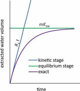
Passive sampler calibration is often done by exposing samplers to a constant concentration of target compounds (C_w), followed by fitting the accumulated amounts to a kinetic model. In many cases it can be assumed that the accumulation rate (dN/dt) is linearly proportional to the effective concentration difference between the water and the sampler.

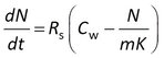
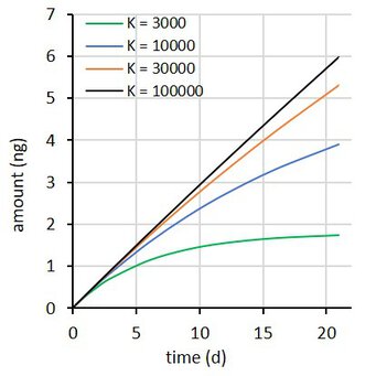
where R_s is the water sampling rate, C_w is the concentration in water, m the sorbent mass, and K the sorbent-water sorption coefficient. This is a first order differential equation. Sampling rate models predict that the difference between the initial and the final concentration in the sampler decays exponentially with time (at constant C_w). Some examples are shown at the right for compounds with K = 3×10³ to 1×10⁵ L/kg, with C_w = 2 ng/L, sorbent mass = 0.0003 kg, and sampling rate (R_s) = 0.15 L/d.

Several variants of passive sampling rate model fits exist.

Model 1: R_s – K model

The model that is easiest to interpret has the water sampling rate (R_s) and the sorption coefficient (K) as adjustable parameters.

This model is sometimes expressed differently, depending on the data processing prior to statistical analysis. Some researchers model the concentration in the sampler (C_s) instead of the amount, and divide both sides of the above equation by the sorbent mass m

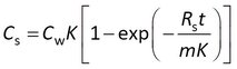
Others first express the data as a concentration factor CF = C_s/C_w

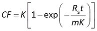
In all of these cases the accumulation data are modeled with R_s and K as adjustable parameters.

Model 2: k_e – K  model

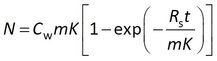
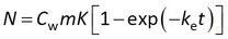
Although model 1 can be fitted to experimental data directly (e.g., R-project, Matlab, and other), some statistics software requires basic transformations in order to match the model with the built-in equations. A frequently used transformation is to write the group R_s /(mK) as a rate constant k_e.

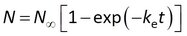
This model can be written in terms of C_s and CF as above, and in addition it can be noted that the accumulated amounts reach a plateau value of N_∞ = C_wmK at equilibrium

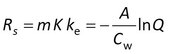
This is the ”one-phase association” standard model in Graphpad Prism. After fitting the data, R_s is obtained from k_e by

R_s = m K k_e

and K is evaluated from

K = N_∞/(mC_w)

A difference with Model 1 is that K and k_e are treated as independent adjustable parameters in the curve fitting. This causes some difficulties because k_e is inversely proportional to K.

Model 3: asymptotic regression model (ABQ model)

Townsend et al. (2018) included an initial amount N₀ in model 2, and rearranged this model to

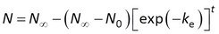
The accumulation data could then be fitted to GenStat’s standard asymptotic regression function

N = A + B Q^t
A = N_∞
B=-( N_∞ – N₀)
Q = exp(-k_e)

After fitting the data to the model, R_s is obtained from

and K is calculated from

K = A/(mC_w)

A difference with model 2 is that an additional parameter is needed (3 instead of 2), and that Q = exp(−k_e) rather than k_e is used as an adjustable parameter. The parameters A = N_∞ and Q =exp(−k_e) are negatively associated in this model (higher K means higher A and lower Q).

2. R_s and K estimates

A challenge with all three models is how to estimate the parameters when the uptake is essentially linear. This happens when the sorption coefficient is very high (black and amber lines in figure above). A further challenge with models 2 and 3 is that R_s is obtained indirectly: from k_e and K for model 2, and from A and Q for model 3. This may (or may not) result in lower accuracy of the estimated R_s values.

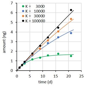
The performance of the models was therefore evaluated by simulating the uptake of three compounds over a time period of 21 d.
Accumulated amounts were calculated from model 1, with K between 3×10³ and 1×10⁵ L/kg, C_w = 2 ng/L, m = 0.0003 kg, and R_s = 0.15 L/d, for 8 exposure times up to 21 d.
A the end of the exposure period the amounts were 97, 65, 30, and 10% of their equilibrium values. For each compound 100 uptake experiments were simulated by adding 5% random noise to the amounts. See adjacent plot for some examples.

Parameters were estimated for models 1, 2, and 3 using weighted nonlinear least squares analysis (R-project, nls function). Parameters were also estimated using Excel’s Solver Add-In (Billo, 2001).

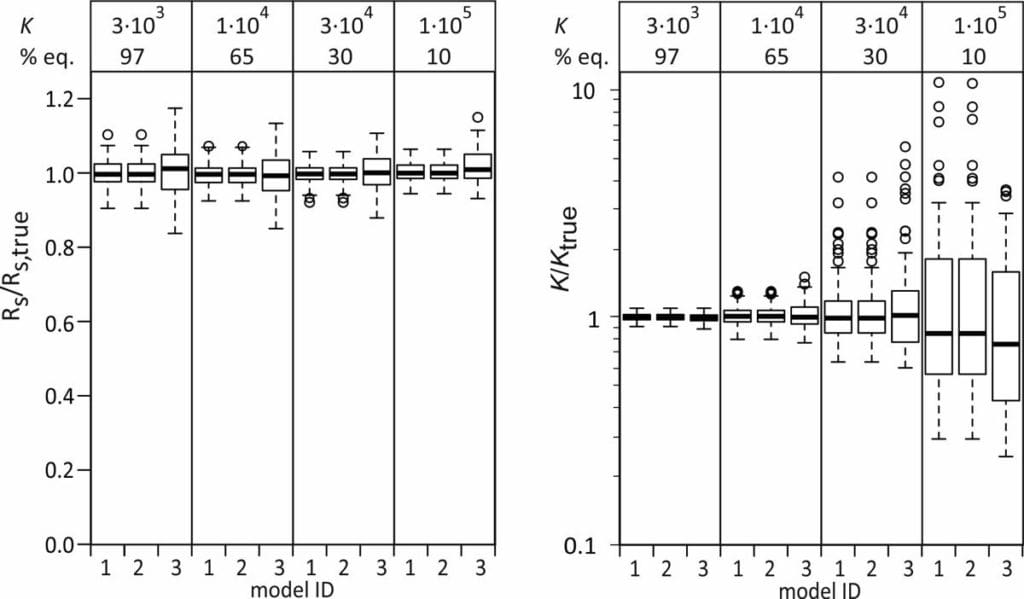
Ratios of estimated and true R_s were close to 1 for all models and all model compounds, even though the R_s estimates from models 2 and 3 were obtained indirectly. The R_s estimates from model 3 show a slightly larger scatter.

Median ratios of estimated and true K values are also close to 1 for all three models. The scatter in the K/K_true ratios is larger for the more linear uptake data, as expected.

3. Uncertainty estimates in R_s and K

Nonlinear least squares analysis includes estimation of the standard errors in the adjustable parameters. R_s is estimated directly with model 1, but is calculated from two other parameters with model 2 (R_s = m K k_e ) and model 3 (R_s = -[A lnQ]/C_w). The usual method for estimating standard errors in calculated values is error propagation under the assumption that the estimated parameters are uncorrelated. The standard error s_Rs is then given for model 2 as

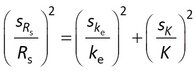
where s_ke and s_K are the standard errors in k_e and K.

Assuming that the error in C_w can be neglected, s_Rs for model 3 is obtained from

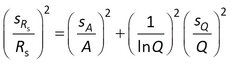
where s_A and s_Q are the standard errors in A and Q.

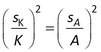
Standard errors in the sorption coefficient (s_K) are obtained directly from the nonlinear least squares output of model 2, and for model 3 s_K is given by

To test the validity of these error estimates, the predicted standard errors in R_s and K for individual model runs (s_predicted) were compared with the observed standard errors within each set of 100 runs (s_observed).  

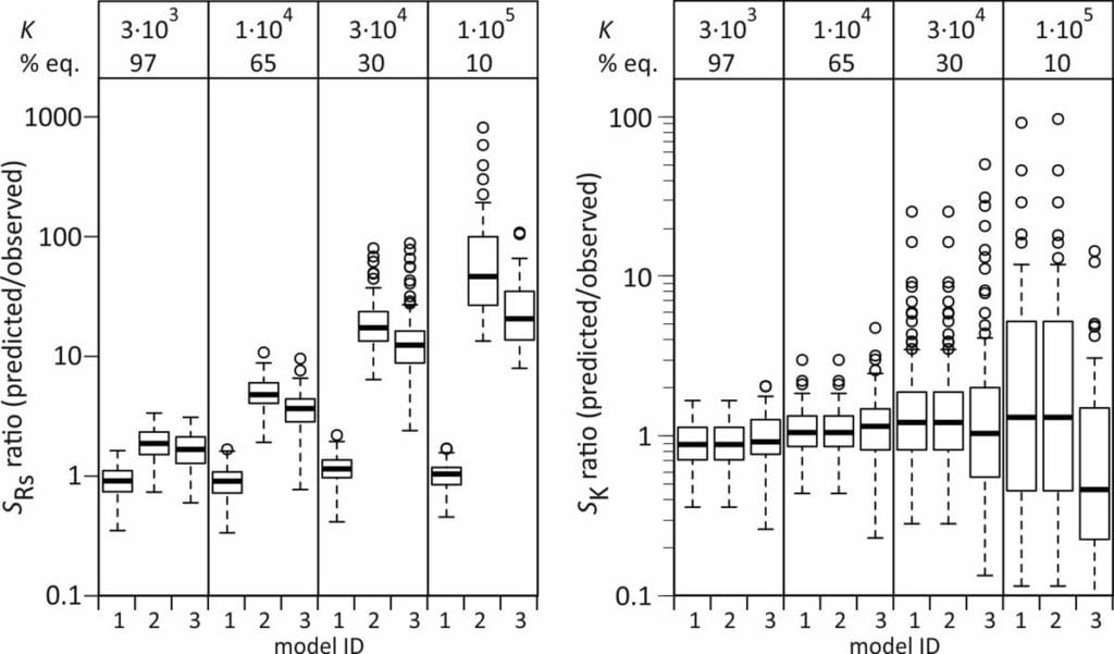
Standard errors in R_s are well-predicted with model 1, but are overestimated with models 2 and 3, also for the compound that reaches 97% equilibrium. Standard errors in K are on average well predicted by all three models, but (naturally) show a large scatter for the compounds that reach a small degree of equilibrium during the exposure.

Better estimates of s_Rs from models 2 and 3 can be obtained by accounting for the covariance between k_e and K (model 2) or A and Q (model 3), but this increases the computational burden, and using model 1 is a more straightforward approach.

4. Choosing nonlinear versus linear least-squares

Nonlinear least squares analysis yields the correct R_s, even when the uptake is essentially linear (see R_s/R_s,true plot above). A practical approach for selecting linear versus nonlinear least squares is to select the method that yields the smallest residual errors. A visual inspection of plots with experimental values and model fit, and a comparison of R_s estimates and standard errors from linear and nonlinear least squares suffices. Alternatively, a partial F-test can be used to check if the nonlinear model (two parameters) gives a significantly better fit than the linear model (one parameter).

Nonlinear least squares estimations do not always converge when the uptake is linear. In those cases the linear model can be selected, again after checking the plots with measured and modeled data.

5. Optimal passive sampling rate model fit

• All three nonlinear models yield similar values of R_s and K
• Only model 1 gives a realistic estimate of the standard error in R_s.
• Choosing between nonlinear and linear model is not very critical. The choice can be based on visual inspection of plots of modeled and experimental data, or on a partial F-test.

6. Free template for the R_s – K model

An excel template for estimation of R_s and K can be downloaded for free. It is easy to operate, and comes with a manual including screenshots.

• Download template manual (pdf)
• Download calculation template manual (xlsx)

Basic features are

• estimates of R_s and K for 10 data sets in one run
• standard errors of R_s and K
• comparison with linear regression results
• partial F-test for choosing nonlinear versus linear modeling
• plots of residual errors
• plots of data + model fit
• weighted and unweighted nonlinear regression
• no macro’s; no security issues
• up to 20 data points per experiment

7. Need to test a different model?

PaSOC is happy to adapt the free passive sampling rate model fit template according you your needs.

• Include a lag phase
• Change the dependent variable from amount to concentration in the sorbent (C_s = N/m) or concentration factor (CF = C_s/C_w)
• Optimize logK instead of K
• Any other modification

Click How we work for further details.

References

Billo, E.J., 2001. Non-linear regression using the solver. In: Excel for Chemists: A Comprehensive Guide. John Wiley & Sons, Inc., New York, pp. 223–238.

Townsend, I., Jones, L., Broom, M., Gravell, A., Schumacher, M., Fones, G.R., Greenwood, R., Mills, G.A., 2018. Calibration and application of the Chemcatcher® passive sampler for monitoring acidic herbicides in the River Exe, UK catchment. Environ. Sci. Pollut. Res. 25, 25130–25142. https://doi.org/10.1007/s11356-018-2556-3

… and embedded URLs in the text

Passive or active?

Consider speciation, temporal variability, uncertainties, detection limits, stratification, and cost, when weighing passive versus active water sampling. Each method has its pros and cons.

With active sampling a well-defined water volume is isolated from the environment and quantitatively extracted. Active sampling comprises grab sampling at high or low temporal resolution, composite sampling, and continuous water sampling with autosamplers. Concentrations are calculated from extracted amounts and the water volume.

With passive sampling a sorption phase is exposed to water in situ. Transport of the target compound to the sorption phase is by diffusion and advection. Concentrations in water are calculated from the accumulated amounts and an accumulation model.

Here are some aspects to consider.

1. Speciation

Nonpolar organic compounds (for example benzo[a]pyrene) can be bound to suspended and dissolved organic matter, but the freely dissolved fraction is a more relevant proxy for bioaccumulation and toxicity at the lower trophic levels of the food web. For polar organic compounds (for example caffeine, carbamazepine) or volatile organic compounds (for example trichloroethene) speciation is not an issue, as sorption to suspended matter is minimal.

Passive and active sampling often give a different type of information

• Passive samplers target the freely dissolved fraction, because the uptake is driven by the difference in chemical activity of the target compound between sorbent and water.
• Active samplers target total concentrations. When a filtration or centrifugation step is included, a further separation can be made between concentrations in suspended matter on one hand, and concentrations of freely dissolved + colloidally bound compounds on the other.

Total concentrations can be relevant when the purpose of the monitoring study is to calculate loads that are carried by a river. Chemical activities are more relevant for risk assessment. Chemical activities can be calculated from total concentrations and vice versa, but this additional modeling comes at the price of reduced accuracy.

Key question 1:
Does the target compound bind significantly to suspended and dissolved organic matter?

• If not: both active and passive sampling can be considered.
• If so: then it depends if you want to know the total concentrations in a water sample (use active sampling) or if you are interested in the chemical activity of the compound in the water sample (use passive sampling).

2. Temporal variability

Concentrations of chemicals can vary with time, and the sampling method should yield a representative picture of compound concentrations for the time frame of interest. Nonpolar legacy contaminants often show a smooth seasonal variation that can be captured by low-frequency active sampling. Concentrations of polar agricultural chemicals and pharmaceuticals vary substantially on the time scale of days or hours (Mutzner et al., 2019; Ort et al., 2010). For these compounds low-frequency grab sampling carries a large sampling uncertainty because the sample can be taken within or between peak concentrations events. Increasing the sampling frequency can be option, but increases labor cost (high-frequency grab sampling) or equipment cost (continuous water sampling). Passive samplers are suitable for time integrated sampling over periods of days, weeks, months, depending on the sampler type and the target compound.

Key question 2:
Are concentrations of target compounds highly variable within the time frame of interest?

• If not: both low-frequency active sampling and passive sampling can be considered.
• If so: high-frequency active sampling and passive sampling can be considered.

3. Stratification

Concentrations in ground water wells may show strong vertical concentration gradients. Active sampling can distort the vertical distributions when water near the sampling inlet is withdrawn (ITRC, 2007). Gradient distortion may also occur for monitoring in the hyporheic zone of rivers (Mechelke et al., 2019). Passive samplers do not draw any water, and therefore do not induce mixing with adjacent water layers, except during deployment.

Key question 3:
Will taking a water sample distort concentration distributions?

• If not: active sampling and passive sampling can both be considered.
• If so: passive sampling is the only way to go.

4. Detection limits

To check if passive samplers meet the required method detection limits it is useful to know the water volume that is extracted after some time. At the initial stage of the sampler deployment this equivalent water volume equals sampling rate x time (R_st). As an example: atrazine sampling rate with Chemcatchers is ~0.13 L/d, and a 3-weeks exposure would extract a water volume of 2.7 L. When, for example, a minimum amount of 1 ng is needed to positively identify the occurrence of atrazine in the environment, then the detection limit would be 1/2.7=0.4 ng/L.

The extracted water volume is however bound to a maximum that occurs when target compounds attain sampler-water equilibrium. In this case the equivalent extracted water volume equals sorbent-mass × sorption-coefficient (mK_sw). As an example: the silicone-water sorption coefficient of pyrene is ~48,000 L/kg. For a silicone strip of 3 g the maximum water volume that can be extracted equals 48,000 × 0.003 = 144 L, which is not easily achieved with active water sampling.

For an initial estimate of the extracted water volume in passive sampling it suffices to calculate R_st and mK_sw , and adopt the smaller of these two values, as illustrated in the figure above.

Sorption coefficients are sometimes not available because no measurable degree of equilibrium is attained in sampler calibration studies. In this case the sorbent acts as an infinite sink, and accumulated amounts increase linearly with time. The calibration data should be inspected to verify the exposure time for which accumulation is linear, and the extracted water volume can be estimated from R_st alone (mK_sw is essentially infinite).  

Key question 4:
Does passive sampling meet the required detection limits?

• If not: consider longer passive sampler exposure times, or alternative passive sampler designs, or stick to active sampling methods.
• If so: passive sampling can be considered.

5. Passive sampler modeling

Uptake models are used to calculate compound concentrations from the amounts that are accumulated by passive samplers. The uptake kinetics of nonpolar compounds by silicone and low-density polyethylene is well understood, including the effects of temperature and flow (Lohmann, 2012; Smedes and Booij, 2012), and the model uncertainties can be obtained from error propagation. Uptake modeling of polar compounds by o-DGT also has a strong mechanistic basis (Challis et al., 2016).

Sampling rates by POCIS and Chemcatcher are less well understood (Charriau et al., 2016; Harman et al., 2012). Model uncertainties can only be derived from the consistency of reported sampling rates for these samplers (Poulier et al., 2014). There are many other passive sampler designs for which model uncertainty is hard to assess because only limited data for calibration and field testing are available.

Key question 5:
Does the uptake model for passive sampler of choice have a strong mechanistic basis, and are the relevant calibration parameters consistent among different studies?

• If not: Further field validation using passive sampling with simultaneous active sampling is needed.
• If so: passive sampling can be considered.

6. Cost

Whether passive or active sampling is cheaper depends on many aspects, such as active sampling frequency and pooling strategy, risk of passive sampler theft or vandalism, speciation issues, and required accuracy. Including field validation of active versus passive sampling at one or more monitoring sites increases confidence in the data, but comes at additional cost. Aspects to include are the cost of labor, chemical analysis, and equipment, and the cost and risk of making incorrect management decisions based on unreliable data.

Key question 6:
Is cost an issue?

• If not: High-frequency active sampling is likely the best option for polar organic compounds. For nonpolar compounds it depends if total concentrations are targeted (contaminant load assessment; best done by high-frequency active sampling) or if freely dissolved concentrations are more relevant (risk assessment; best done by passive sampling).
• If so: a further cost-benefit analysis is needed to make an optimal choice between passive and active sampling.

Send your comments and questions

The above covers the main lines of choosing passive versus active water sampling. When you are short of time, PaSOC is happy to make a more detailed analysis of your specific monitoring requirements. Click How we work for further details.

At your service.

Further reading

Castle, G.D., Mills, G.A., Bakir, A., Gravell, A., Schumacher, M., Townsend, I., Jones, L., Greenwood, R., Knott, S., Fones, G.R., 2018. Calibration and field evaluation of the Chemcatcher® passive sampler for monitoring metaldehyde in surface water. Talanta 179, 57–63. https://doi.org/10.1016/j.talanta.2017.10.053

Challis, J.K., Hanson, M.L., Wong, C.S., 2016. Development and calibration of an organic-diffusive gradients in thin films aquatic passive sampler for a diverse suite of polar organic contaminants. Anal. Chem. 88, 10583–10591. https://doi.org/10.1021/acs.analchem.6b02749

Charriau, A., Lissalde, S., Poulier, G., Mazzella, N., Buzier, R., Guibaud, G., 2016. Overview of the Chemcatcher® for the passive sampling of various pollutants in aquatic environments Part A: Principles, calibration, preparation and analysis of the sampler. Talanta 148, 556–571. https://doi.org/10.1016/j.talanta.2015.06.064

Harman, C., Allan, I.J., Vermeirssen, E.L.M., 2012. Calibration and use of the polar organic chemical integrative sampler – a critical review. Environ. Toxicol. Chem. 31, 2724–2738. https://doi.org/10.1002/etc.2011

ITRC, 2007. Protocol for use of five passive samplers to sample for a variety of contaminants in groundwater (DSP-5). Interstate Technology & Regulatory Council, Washington, DC 20001. https://www.itrcweb.org/GuidanceDocuments/DSP-5.pdf

Lohmann, R., 2012. Critical review of low-density polyethylene’s partitioning and diffusion coefficients for trace organic contaminants and implications for its use as a passive sampler. Environ. Sci. Technol. 46, 606–618. https://doi.org/10.1021/es202702y

Mechelke, J., Vermeirssen, E.L.M., Hollender, J., 2019. Passive sampling of organic contaminants across the water-sediment interface of an urban stream. Water Res. 165, 114966. https://doi.org/10.1016/j.watres.2019.114966

Mutzner, L., Vermeirssen, E.L.M., Ort, C., 2019. Passive samplers in sewers and rivers with highly fluctuating micropollutant concentrations – Better than we thought. J. Hazard. Mater. 361, 312–320. https://doi.org/10.1016/j.jhazmat.2018.07.040

Ort, C., Lawrence, M.G., Reungoat, J., Mueller, J.F., 2010. Sampling for PPCPs in wastewater systems: comparison of different sampling modes and optimization strategies. Environ. Sci. Technol. 44, 6289–6296. https://doi.org/10.1021/es100778d

Poulier, G., Lissalde, S., Charriau, A., Buzier, R., Delmas, F., Gery, K., Moreira, A., Guibaud, G., Mazzella, N., 2014. Can POCIS be used in Water Framework Directive (2000/60/EC) monitoring networks? A study focusing on pesticides in a French agricultural watershed. Sci. Total Environ. 497–498, 282–292. https://doi.org/10.1016/j.scitotenv.2014.08.001

Smedes, F., Booij, K., 2012. Guidelines for passive sampling of hydrophobic contaminants in water using silicone rubber samplers. (No. ICES Techniques in Marine Environmental Sciences 52.). International Council for the Exploration of the Sea, Copenhagen. https://dx.doi.org/10.17895/ices.pub.5077